Diffusion Analysis in a Pore (MC Method)
The MC diffusion analysis needs the sampled object file using the mc diffusion routine
import porems as pms
import poreana as pa
import matplotlib.pyplot as plt


# Load molecule
mol = pms.Molecule("benzene", "BEN", inp="data/benzene.gro")

# Set step length
len_steps = [1,2,5,10,20,30,40]

# Set frame length
len_frame = 2e-12

# Sample transition matrix
sample = pa.Sample("data/pore_system_cylinder.obj", "data/traj_cylinder.xtc", mol)
sample.init_diffusion_mc("output/diff_mc_cyl_s.h5", len_steps, len_frame=len_frame)
sample.sample(is_parallel=False)
Finished frame 2001/2001...
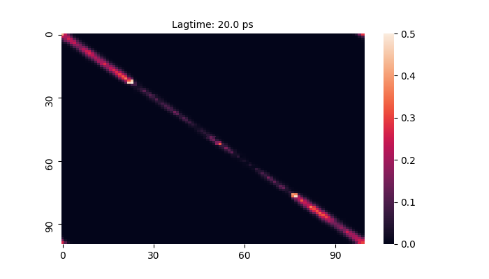
With the sampling obj-file the transition matrix can be plotted
# Set kwargs for the heatmap
kwargs = {"vmin":0,"vmax":0.5, "xticklabels":30, "yticklabels":30, "cbar":True, "square":False}

# Plot transition matrix for a step length of 10
pa.diffusion.mc_trans_mat("output/diff_mc_cyl_s.h5", 10, kwargs)
After sampling, a model has to set and the MC Alogirthm started
# Set Cosine Model for diffusion and energy profile
model = pa.CosineModel("output/diff_mc_cyl_s.h5", 6, 10)

# Do the MC Algorithm
pa.MC().run(model,"output/diff_mc.h5", nmc_eq=5000, nmc=5000, print_output=False, is_parallel=False)
MC Calculation Start
...
MC Calculation Done.
The results of the MC Alogrithm the diffusion can be calculated
# Print the results for the normal diffusion
diff,diff_mean,diff_table = pa.diffusion.mc_fit("output/diff_mc.h5")
Diffusion axial: 1.6913e-09 m^2/s
Mean Diffusion axial: 1.6777e-09 m^2/s
Standard deviation: 6.9341e-11 m^2/s

or the diffusion and free energy profile over the entire system can be displayed
# Plot diffusion profile over the simulation box
pa.diffusion.mc_profile("output/diff_mc.h5", infty_profile=True)

# Plot free energy profile over the simulation box
pa.freeenergy.mc_profile("output/diff_mc.h5", [10])

Additionally, the pore area can be considered more closely
# Plot the lag time extrapolation for the pore ares
pa.diffusion.mc_fit("output/diff_mc.h5", section="pore")

# Plot diffusion profile in a pore
pa.diffusion.mc_profile("output/diff_mc.h5", section="pore", infty_profile=True)
Diffusion axial (Pore): 1.2534e-09 m^2/s
Mean Diffusion axial (Pore): 1.3417e-09 m^2/s
Standard deviation: 3.1949e-10 m^2/s
