Simulation Workflow
In this workflow a simply simulation system will be generated and analyzed. After installing the package via PyPI
pip install simemobilecity
it can be imported into the python script
import simemobilecity as sec
Create Topology
First, the topology object is generated by loading the OSM map using an OSMnx wrapper function
name = "Munich, Bavaria , Germany"
topo = sec.Topology({"name": name})
Since this step takes a long time depending on the complexity of the desired map, it is advised to deposit the graph objects for later use
sec.utils.save(topo.get_G(), "data/munich_G.obj")
sec.utils.save(topo.get_Gp(), "data/munich_Gp.obj")
The save functionality creates pickle object files containing the graph \(G\) and the projected graph \(G_p\), necessary for running the simulation. Once saved, the object files can be loaded later
G = sec.utils.load("data/munich_G.obj")
Gp = sec.utils.load("data/munich_Gp.obj")
topo = sec.Topology({"name": name, "G": G, "Gp": Gp})
Define User and POI objects
The next step is defining the user and POI objects which contain the probability densities for charging sessions.
input_all = 0.2
input_daily = {0: 0.0, 1: 0.1, 2: 0.2, 3: 0.3, 4: 0.4, 5: 0.5, 6: 0.6}
input_hourly = { 0: 0.0,  1: 0.1,  2: 0.2,  3: 0.3,  4: 0.4,  5: 0.5,  6: 0.6,  7: 0.7,  8: 0.8,  9: 0.9, 10: 0.0, 11: 0.1,
                12: 0.2, 13: 0.3, 14: 0.4, 15: 0.5, 16: 0.6, 17: 0.7, 18: 0.8, 19: 0.9, 20: 0.0, 21: 0.1, 22: 0.2, 23: 0.3}
input_exact = {0: { 0: 0.0,  1: 0.1,  2: 0.2,  3: 0.3,  4: 0.4,  5: 0.5,  6: 0.6,  7: 0.7,  8: 0.8,  9: 0.9, 10: 0.0, 11: 0.1,
                   12: 0.2, 13: 0.3, 14: 0.4, 15: 0.5, 16: 0.6, 17: 0.7, 18: 0.8, 19: 0.9, 20: 0.0, 21: 0.1, 22: 0.2, 23: 0.3},
               1: { 0: 0.0,  1: 0.1,  2: 0.2,  3: 0.3,  4: 0.4,  5: 0.5,  6: 0.6,  7: 0.7,  8: 0.8,  9: 0.9, 10: 0.0, 11: 0.1,
                   12: 0.2, 13: 0.3, 14: 0.4, 15: 0.5, 16: 0.6, 17: 0.7, 18: 0.8, 19: 0.9, 20: 0.0, 21: 0.1, 22: 0.2, 23: 0.3},
               2: { 0: 0.0,  1: 0.1,  2: 0.2,  3: 0.3,  4: 0.4,  5: 0.5,  6: 0.6,  7: 0.7,  8: 0.8,  9: 0.9, 10: 0.0, 11: 0.1,
                   12: 0.2, 13: 0.3, 14: 0.4, 15: 0.5, 16: 0.6, 17: 0.7, 18: 0.8, 19: 0.9, 20: 0.0, 21: 0.1, 22: 0.2, 23: 0.3},
               3: { 0: 0.0,  1: 0.1,  2: 0.2,  3: 0.3,  4: 0.4,  5: 0.5,  6: 0.6,  7: 0.7,  8: 0.8,  9: 0.9, 10: 0.0, 11: 0.1,
                   12: 0.2, 13: 0.3, 14: 0.4, 15: 0.5, 16: 0.6, 17: 0.7, 18: 0.8, 19: 0.9, 20: 0.0, 21: 0.1, 22: 0.2, 23: 0.3},
               4: { 0: 0.0,  1: 0.1,  2: 0.2,  3: 0.3,  4: 0.4,  5: 0.5,  6: 0.6,  7: 0.7,  8: 0.8,  9: 0.9, 10: 0.0, 11: 0.1,
                   12: 0.2, 13: 0.3, 14: 0.4, 15: 0.5, 16: 0.6, 17: 0.7, 18: 0.8, 19: 0.9, 20: 0.0, 21: 0.1, 22: 0.2, 23: 0.3},
               5: { 0: 0.0,  1: 0.1,  2: 0.2,  3: 0.3,  4: 0.4,  5: 0.5,  6: 0.6,  7: 0.7,  8: 0.8,  9: 0.9, 10: 0.0, 11: 0.1,
                   12: 0.2, 13: 0.3, 14: 0.4, 15: 0.5, 16: 0.6, 17: 0.7, 18: 0.8, 19: 0.9, 20: 0.0, 21: 0.1, 22: 0.2, 23: 0.3},
               6: { 0: 0.0,  1: 0.1,  2: 0.2,  3: 0.3,  4: 0.4,  5: 0.5,  6: 0.6,  7: 0.7,  8: 0.8,  9: 0.9, 10: 0.0, 11: 0.1,
                   12: 0.2, 13: 0.3, 14: 0.4, 15: 0.5, 16: 0.6, 17: 0.7, 18: 0.8, 19: 0.9, 20: 0.0, 21: 0.1, 22: 0.2, 23: 0.3}}
Therefore multiple input possibilities exist
- input_all - Sets the probability for all hours of all days to the same value
- input_daily - Sets a different probability for all hours of each day
- input_hourly - Sets the same probability for all days for each hour
- input_exact - Sets a different probability for each hour for each day
These probability inputs are then passed to the object constructures of the User
user_a = sec.User(input_hourly)
user_b = sec.User(input_exact)
and POI classes
poi_a = sec.Poi(topo, {"amenity": ["cafe"]}, input_all)
poi_b = sec.Poi(topo, {"amenity": ["restaurant"]}, input_daily)

topo.plot(pois=[topo.poi({"amenity": ["cafe"]})])
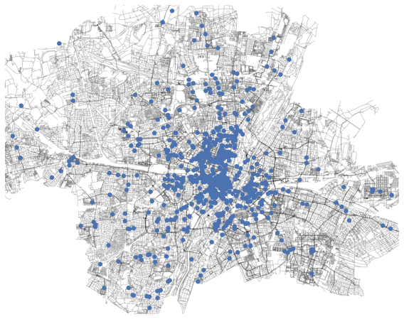
In case of the POIs, a description tag is added for extracting the relevant POIs. A list of available tags is available on the OSM website.
Simulation
Finally, the simulation is run using the Monte Carlo class by first adding the user and POI objects, then defining the simulation parameters at the execution command
mc = sec.MC(topo)
mc.add_user(user_a, 50)
mc.add_user(user_b, 50)
mc.add_poi(poi_a)
mc.add_poi(poi_b)
mc.set_drivers(100)
traj = mc.run("data/traj.obj", weeks=4, weeks_equi=1)
Starting preparation...
Starting equilibration...
Finished day 7/7...
Starting production...
Finished day 28/28...
The definition of the number of drivers is analogous to the definitions of the probabilities shown earlier.
Optimization
Once the simulation is finished, the output trajectory can be analyzed using the Optimize module
opt = sec.Optimize(topo)
capacity_opt = opt.run("data/opt.obj", traj, crit={"dist": 0.85, "occ": 0.05})
Finished node 430/430...
This new optimized charging station list can be passed to the MC class for further iterations
traj_opt = mc.run("data/traj_opt.obj", weeks=4, weeks_equi=1, capacity=capacity_opt)
Analysis
The simulated data can be extracted using the trajectory functionalities
extract = traj["cs"].extract(days=list(range(7)), hours=list(range(24)), users=list(range(2)), is_norm=False)
This command aggregates the data of all days, all hours, and all users of all nodes into a single data structure. The necessary data is converted into a pandas Dataframe
import pandas as pd

data = [{"node": node, "x": G.nodes[node]["x"], "y": G.nodes[node]["y"], "Charging Sessions": x["success"], "Occupancy Fail": x["fail"]["occ"], "Distance Fail": x["fail"]["dist"]} for node, x in extract.items()]
df = pd.DataFrame(data)
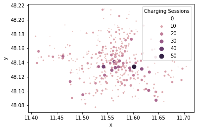
and then plotted using the scatterplot function of seaborn
import seaborn as sns

sns.scatterplot(data=df, x="x", y="y", hue="Charging Sessions", size="Charging Sessions")
Note
For further information, more thorough variable descriptions and functionalities, visit the API section of this documentation website.